Supported Control Chart Types
This page summarises the available control chart types and their implementation. For any other chart types that you’d like to see added, please open an issue on the GitHub page.
Why SPC?
Statistical Process Control (SPC) is a method for monitoring changes in a given outcome over time, and identifying whether a given change is large enough to be considered statistically meaningful.
Originally introduced for monitoring manufacturing processes, SPC has become a key approach for monitoring healthcare outcomes over time.
Choosing a Chart Type
There are multiple types of SPC charts, each for monitoring a different type of data.
If you are unsure of which chart type would be most appropriate for your use-case, you can use this flow-chart to guide you.
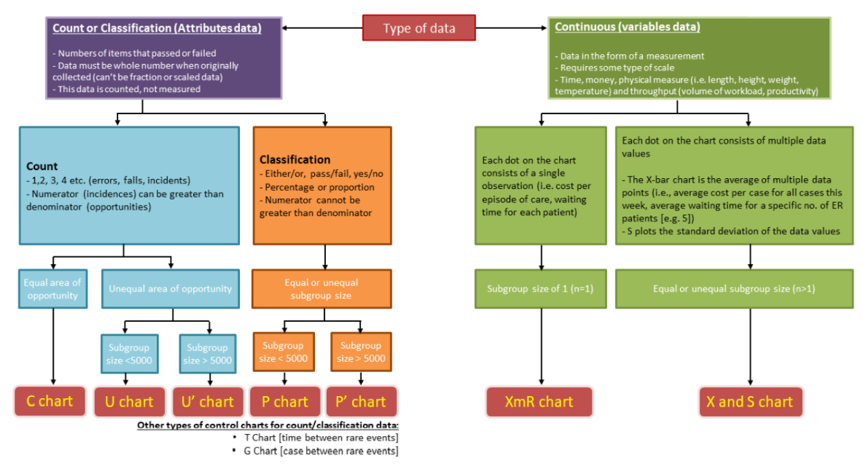
Adapted from: https://qi.elft.nhs.uk/wp-content/uploads/2020/03/how-to-use-statistical-process-control-spc-charts.pdf
Calculating 3-sigma limits
The functions for calculating 3-sigma limits are consistent with the R package qicharts2, and are based on the formulas provided by Montgomery (2009), Introduction to Statistical Quality Control.
Generally, the model for calculating the lower and upper control limits for SPC charts is:
\[\begin{aligned} \bar{x} \pm 3SD \end{aligned}\]where \(\bar{x}\) is the weighted average of the sample statistic and \(SD\) is the weighted sample standard deviation.
Each of the chart types have different probability models, and thus the calculation of the control limits differs between them.
| Chart Type | Assumed Distribution | Control Limits | Assumptions |
|---|---|---|---|
| i | Gaussian | \(\bar{x} \pm 2.66 \overline{MR}\) | \(\bar{x}\) is the sample average, \(\overline{MR}\) is the average moving range of successive observations |
| mr | Gaussian | \(3.267 \overline{MR}\) | \(\overline{MR}\) is the average moving range (no lower 3-sigma limit) |
| p | Binomial | \(\bar{p} \pm 3\sqrt{\frac{\bar{p}(1-\bar{p})}{p_1}}\) | \(\bar{p}\) is the average number of defectives, \(n_i\) is the sample size |
| u | Poisson | \(\bar{u} \pm 3\sqrt{\frac{\bar{u}}{n_i}}\) | \(\bar{u}\) is the average number of defects per unit, \(n_i\) is the size of inspection unit |
| c | Poisson | \(\bar{c} \pm 3\sqrt{\bar{c}}\) | \(\bar{c}\) is the average number of defects |
| xbar | Gaussian | \(\bar{x} \pm A_3 \bar{s}\) | \(\bar{x}\) is the sample average, \(A_3\) is a constant depending on the sample size, \(\bar{s}\) is the weighted sample standard deviation |
| s | Gaussian | \(CL = \bar{s}, \newline LCL = B_3 \bar{s}, \newline UCL = B_4 \bar{s}\) | \(\bar{s}\) is the weighted sample standard deviation, \(B_3\) and \(B_4\) are constants depending on the sample size |
| g | Geometric | \(\bar{x} \pm 3\sqrt{\bar{x}(\bar{x} + 1)}\) | \(\bar{x}\) is the average number of opportunities between events |
The \(p'\) and \(u'\) charts are based upon the above assumptions for \(p\) and \(u\) charts, however they account for Laney’s correction factor for prime charts from Laney 2002, Improved Control Charts for Attributes.
The \(t\) chart three sigma limits are calculated by the \(i\) chart method applied on the transformed data. Where \(y\) is the time between events, it is transformed to \(y^{1/3.6}\) and the \(i\) chart is applied. The limits are then back transformed (\(cl = cl^{3.6}\)).